From Lincoln-Petersen to the Cormack-Jolly-Seber Model

Author

Deon Roos

Published

March 4, 2026

A local hero (two of them, actually)

Before we get into the model, I want to take a moment to point something out that I think is genuinely worth appreciating.

The Cormack-Jolly-Seber model, or CJS model, is one of the most widely used statistical models in ecology. It underpins decades of research into animal survival, population dynamics, and conservation. If you have ever read a paper reporting survival estimates for a wild animal population, there is a very good chance CJS was involved somewhere.

Richard Cormack and George Jolly both developed this model in 1964. Both were working at the University of Aberdeen, in the ARC Unit of Statistics. They worked in the same corridor. They had coffee together most mornings. They even played chess together regularly (specifically a version of chess called kriegspiel which is kind of like battleships + chess).

And neither had any idea the other was working on the same problem.

Cormack later recalled that it was “completely unknown to the two of us that we were working in the same area.” They were sitting across a chess board from each other and somehow the topic of mark-recapture never came up. It was only when Cormack submitted his paper to Biometrika in 1964 that the overlap became apparent, through the referee’s comments rather than through any conversation between the two of them.

It’s also worth noting that Cormack went to Cambridge at 17, did his undergraduate in two years, and became a lecturer in Aberdeen at 21…

George Seber developed his version independently in New Zealand at around the same time, which makes three separate derivations of essentially the same model, across two continents, by people who were unaware of each other’s work. Hence all three names on the tin.

So the next time someone asks you what Aberdeen is known for, you have a genuinely good answer. Two of them, actually, sitting in the same corridor, drinking coffee, playing chess, and accidentally doing the same groundbreaking statistics.

What LP could not do

On the previous page we saw that the Lincoln-Petersen estimator gives you a snapshot estimate of population size \(N\) using two sampling occasions and the assumption that the population is closed. No births, no deaths, no movement in or out.

That closure assumption is doing a lot of heavy lifting. It is defensible over short time windows but falls apart the moment your study extends over weeks or months. And if your actual biological question is about survival, closure is not just inconvenient, it is actively the wrong assumption. You want animals to be able to die between occasions, because that is the thing you are trying to estimate.

The CJS (Cormack-Jolly-Seber) model drops the closure assumption entirely. Animals can die between sampling occasions. The population is open. And in exchange for giving up closure, we gain something valuable: an estimate of apparent survival probability \(\phi\).

The trade-off is that we can no longer estimate \(N\) directly. CJS conditions on first capture, meaning it only uses the history of animals after they have been caught at least once. Animals that were never caught do not feature in the model at all. This sidesteps the problem of estimating how many animals were never seen, but it also means \(N\) is off the table.

We will get \(N\) back eventually. That is actually one of the main payoffs of the robust design. But for now, let us build up to CJS carefully.

The capture history

The fundamental data structure in CJS is the capture history. This is something new compared to what you have worked with before, so it is worth spending a moment on it.

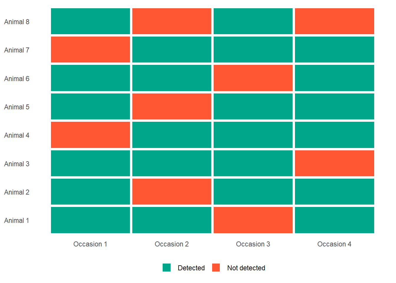
Each tagged animal gets its own row. Each column represents a sampling occasion. A 1 means the animal was detected on that occasion. A 0 means it was not. That is it.

Here is a small example with five animals surveyed over four occasions:

Code

library(ggplot2)
library(dplyr)
library(tidyr)

ch <- data.frame(
  animal = paste0("Animal ", 1:8),
  occ1 = c(1, 1, 1, 0, 1, 1, 0, 1),
  occ2 = c(1, 0, 1, 1, 0, 1, 1, 0),
  occ3 = c(0, 1, 1, 1, 1, 0, 1, 1),
  occ4 = c(1, 1, 0, 1, 1, 1, 1, 0)
)

ch

    animal occ1 occ2 occ3 occ4
1 Animal 1    1    1    0    1
2 Animal 2    1    0    1    1
3 Animal 3    1    1    1    0
4 Animal 4    0    1    1    1
5 Animal 5    1    0    1    1
6 Animal 6    1    1    0    1
7 Animal 7    0    1    1    1
8 Animal 8    1    0    1    0

Read each row as a story. Animal 1 was detected on occasions 1, 2, and 4, but not 3. Animal 2 was detected on 1, 3, and 4, but not 2. And so on.

Now, for each 0 in this table, ask yourself the question from the previous page: is this animal alive and missed, or is it dead? The capture history does not tell you directly. But the pattern across multiple occasions does contain that information, and that is what the CJS model extracts.

Code

ch_long <- ch |>
  pivot_longer(cols = starts_with("occ"),
               names_to = "occasion",
               values_to = "detected") |>
  mutate(occasion = as.integer(gsub("occ", "", occasion)),
         detected_label = if_else(detected == 1, "Detected", "Not detected"))

ggplot(ch_long, aes(x = occasion, y = animal, fill = detected_label)) +
  geom_tile(colour = "white", linewidth = 1.5) +
  scale_fill_manual(values = c("Detected" = "#00A68A",
                                "Not detected" = "#FF5733")) +
  scale_x_continuous(breaks = 1:4, labels = paste("Occasion", 1:4)) +
  labs(x = NULL, y = NULL, fill = NULL) +
  theme_minimal() +
  theme(legend.position = "bottom",
        panel.grid = element_blank())

The green tiles are detections. The red tiles are non-detections. For every red tile, there are two possible stories. The CJS model is a machine for working out which story is more likely, given the full pattern of the data.

Have a look at the figure above. Look at Animal 1 at the bottom. We never caught animal 1 on occasion 3 but we did capture it on occasion 4. We’ve said that non-detection can mean two things; 1) alive but not seen or 2) dead. Was animal 1 dead at occasion 3? Hopefully you conclude it was not, but how do you know? That’s the logic that CJS uses.

The two processes

Just like in the previous page, CJS explicitly models two separate processes:

Process 1: Survival. Between each pair of consecutive occasions, an animal either survives with probability \(\phi\) (e.g. \(0.9\) or 90%) or dies with probability \(1 - \phi\) (e.g. \(1-0.9=0.1\) or 100-90=10%). Once dead, it stays dead. It cannot come back. Zombies don’t exist in this house.

Process 2: Detection. On each occasion, an animal that is alive is detected with probability \(p\), or missed with probability \(1 - p\).

A detection in your data requires both processes to go the right way: the animal must have survived to that occasion, and you must have detected it. A non-detection could be either process failing.

This is the same logic as the previous page, just now written as a model with two explicit parameters.

Building the likelihood from a capture history

Here is where the GLM framing from the first page comes back in. CJS estimates \(\phi\) and \(p\) by writing down the probability of observing each animal’s capture history, and then finding the values of \(\phi\) and \(p\) that make the observed histories as probable as possible. That is maximum likelihood estimation, which you already met in BI3010 (and probably forgot - fair enough).

Let us work through a single animal’s capture history to make this concrete.

Take an animal with history 1 0 1 1. It was caught on occasion 1 (that is how it got tagged), missed on occasion 2, then caught on occasions 3 and 4.

What is the probability of observing this history? Working occasion by occasion after first capture:

Occasion 1 to 2: The animal survived (\(\phi\)) but was not detected (\(1 - p\)). Probability: \(\phi \times (1 - p)\)
Occasion 2 to 3: The animal survived (\(\phi\)) and was detected (\(p\)). Probability: \(\phi \times p\)
Occasion 3 to 4: The animal survived (\(\phi\)) and was detected (\(p\)). Probability: \(\phi \times p\)

Putting it together, the probability of the full history 1 0 1 1 (after first capture) is:

\[P(\text{1 0 1 1}) = [\phi(1-p)] \times [\phi \cdot p] \times [\phi \cdot p]\]

\[= \phi^3 \times p^2 \times (1-p)\]

Code

# Probability of history 1011 as a function of phi and p
phi <- seq(0.01, 0.99, length.out = 100)
p   <- seq(0.01, 0.99, length.out = 100)

grid <- expand.grid(phi = phi, p = p)
grid$prob <- grid$phi^3 * grid$p^2 * (1 - grid$p)

ggplot(grid, aes(x = phi, y = p, fill = prob)) +
  geom_raster() +
  scale_fill_viridis_c(option = "plasma", name = "Probability\nof history") +
  labs(
    x = expression(phi ~ "(survival)"),
    y = "p (detection)",
    title = "Probability of capture history 1 0 1 1",
    subtitle = expression(phi^3 ~ "\u00d7" ~ p^2 ~ "\u00d7" ~ (1 - p))
  ) +
  theme_minimal()

The brighter areas of the plot show combinations of \(\phi\) and \(p\) that make this particular history more probable. Maximum likelihood estimation finds the peak of this surface across all animals simultaneously.

Based on this maximum likelihood estimate, we’d estimate survival as roughly (eye balling the figure above) at something close to 100% and detection as roughly 60%.

But what about the final non-detection?

There is a subtlety I have been glossing over. What if an animal’s last recorded detection is not its last occasion? For example, what about an animal with history 1 1 0 0?

After its last detection on occasion 2, two things could have happened. It could have died at some point before or after occasion 3. Or it could have survived all the way to the end of the study and just never been detected again.

The probability of never being seen again from occasion \(t\) onwards, which is usually written \(\chi_t\) (chi, pronounced “ky”), captures this. For our four-occasion example, \(\chi_4 = 1\) because after the last occasion there are no more chances to be seen. Working backwards:

\[\chi_3 = (1 - \phi) + \phi(1-p)\chi_4\]

In words: the probability of not being seen again from occasion 3 is either the animal died between 3 and 4 (\((1 - \phi)\)) or it survived but was not detected on occasion 4 and then was never seen again (\(\phi(1-p)\chi_4\)).

This recursion continues back through all occasions. CJS handles this automatically, but it is worth knowing it is there, because it is what allows the model to deal honestly with animals that are never recaptured after their first detection.

The model equations

Putting it all together, the CJS model can be written as two linked processes:

\[z_{i,t} \sim Bernoulli(\phi_{t-1} \times z_{i,t-1})\]

\[y_{i,t} \sim Bernoulli(p_t \times z_{i,t})\]

where:

\(z_{i,t}\) is the true alive/dead state of individual \(i\) at occasion \(t\). This is a latent variable: we never observe it directly, we only observe detections.
\(\phi_{t-1}\) is the probability of surviving from occasion \(t-1\) to \(t\)
\(y_{i,t}\) is the observed detection of individual \(i\) at occasion \(t\) (the 0 or 1 in the capture history)
\(p_t\) is the probability of detecting individual \(i\) at occasion \(t\), given it is alive

The first equation says: the true state at time \(t\) is a Bernoulli trial that depends on whether the animal was alive at \(t-1\) and on the survival probability. If the animal is dead (\(z_{i,t-1} = 0\)), it stays dead (\(\phi \times 0 = 0\)). If it is alive, it survives to \(t\) with probability \(\phi\).

The second equation says: what we actually observe is a Bernoulli trial that depends on whether the animal is alive at \(t\) and on the detection probability. You cannot detect a dead animal (\(p \times 0 = 0\)). You detect a live one with probability \(p\).

If these two equations look familiar from the previous page, that is not a coincidence. This is exactly the structure we described in words when we said a detection requires both survival and detectability. We have just written it down formally.

Fitting a CJS model in R

Let us simulate some capture history data and fit a CJS model to it to see this in practice.

Code

set.seed(42)

n_animals <- 100
n_occasions <- 5
phi_true <- 0.80
p_true   <- 0.45

# Simulate true survival states
alive <- matrix(0, nrow = n_animals, ncol = n_occasions)
alive[, 1] <- 1  # All animals alive at first capture

for (t in 2:n_occasions) {
  alive[, t] <- rbinom(n_animals, 1, alive[, t-1] * phi_true)
}

# Simulate detections
detected <- matrix(0, nrow = n_animals, ncol = n_occasions)
for (t in 1:n_occasions) {
  detected[, t] <- rbinom(n_animals, 1, alive[, t] * p_true)
}

# Force first occasion to 1 (all animals were caught at least once to be tagged)
detected[, 1] <- 1

# Show first 10 capture histories
head(detected, 10)

      [,1] [,2] [,3] [,4] [,5]
 [1,]    1    0    0    0    0
 [2,]    1    0    0    0    0
 [3,]    1    1    0    1    0
 [4,]    1    0    0    0    0
 [5,]    1    0    0    0    1
 [6,]    1    1    1    1    1
 [7,]    1    0    0    0    0
 [8,]    1    1    0    0    0
 [9,]    1    0    0    0    0
[10,]    1    1    0    0    0

Now we can fit the CJS model. We will use the marked package, which provides a clean interface for CJS models in R.

Code

library(marked)

# Format as data frame with capture history string
ch_strings <- apply(detected, 1, paste, collapse = "")
cjs_data <- data.frame(ch = ch_strings)

# Fit a simple CJS model with constant phi and p
cjs_fit <- crm(cjs_data,
               model = "CJS",
               model.parameters = list(
                 Phi = list(formula = ~ 1),
                 p   = list(formula = ~ 1)
               ),
               hessian = TRUE)


 Number of evaluations:  100  -2lnl: 404.1465438

Code

cjs_fit


crm Model Summary

Npar :  2
-2lnL:  404.1465
AIC  :  408.1465

Beta
                  Estimate        se        lcl          ucl
Phi.(Intercept)  1.2898696 0.2526289  0.7947169  1.785022249
p.(Intercept)   -0.4241131 0.2133404 -0.8422602 -0.005965891

Code

# Back-transform estimates from logit scale to probability scale
results <- data.frame(
  parameter = c("Survival (phi)", "Detection (p)"),
  true_value = c(phi_true, p_true),
  estimate = plogis(c(cjs_fit$results$beta$Phi,
                      cjs_fit$results$beta$p))
)

results

       parameter true_value  estimate
1 Survival (phi)       0.80 0.7841251
2  Detection (p)       0.45 0.3955330

The estimates should be reassuringly close to the true values we used to simulate the data. They will not be identical because we are working with a finite sample, but they should be in the right ballpark. All this to show that CJS models work.

What CJS gives us, and what it still cannot

CJS is a genuine step forward from Lincoln-Petersen. We now have:

An estimate of apparent survival \(\phi\) that is not contaminated by detection probability
An explicit model for both the biological process (survival) and the observation process (detection)
The ability to use more than two sampling occasions, which gives us more information and more precise estimates
The ability to model \(\phi\) and \(p\) as functions of covariates, just like in a standard GLM

But CJS still has a gap. Because it conditions on first capture and deals only with marked individuals, it cannot estimate \(N\). We lost that when we abandoned the closure assumption.

There is also a subtlety in what \(\phi\) actually represents. CJS is estimated from animals that were captured within your study area and then either recaptured or not. An animal that permanently emigrates looks identical to a dead animal in the capture history. So \(\phi\) is apparent survival: the probability of surviving and remaining within the study area. True survival is higher, by some unknown amount that depends on how much emigration there is.

So we have survival but no population size. We have population size under closure (LP) but no survival. What we really want is both, simultaneously, from the same dataset.

That is exactly what the robust design delivers. And the way it does it is by being clever about the time structure of sampling, nesting closed sampling occasions inside an open population framework.

That is the next page.