Implementing the Robust Design in RMark

Putting it all together

Up to this point we have built up the robust design from first principles. You know what the model is doing, why it needs two time scales, what the parameters mean, and where the ambiguous zeros live. Now we need to actually use it on data.

This page is deliberately practical. Less theory, more code. By the end you should be able to take a real robust design dataset, organise it correctly, specify and fit a model with covariates, and produce figures that communicate what you found.

We will keep using RMark throughout. As a reminder, RMark is an R interface to program MARK, which needs to be installed separately. If you have not done that yet, you can find it here.

What should influence your parameters?

Before you fit any model, you need to think carefully about what covariates to include and in which part of the model. This is not a statistical question, it is a biological one, and getting it wrong at this stage means your model will not reflect reality no matter how well it runs.

There are four parameters in the full robust design model, and each has a different biological interpretation that should guide your covariate choices.

What influences survival (\(\phi\))?

Survival is estimated between primary periods, so the covariates that make sense here are things that vary between primary periods and plausibly affect whether an animal lives or dies.

Body condition is the classic example. An animal in poor condition going into winter is less likely to survive to spring. Age matters for most species, with survival often lower in juveniles and very old individuals. Sex can matter if males and females face different predation or energetic pressures. Environmental conditions between primary periods, such as winter severity, drought intensity, or food availability, are commonly included. If you have interventions, such as supplementary feeding, a predator removal programme, or a disease treatment, those belong here too.

The key question to ask yourself is: between my sampling occasions, what determined whether an animal was alive or dead at the next one?

What influences detection (\(p\))?

Detection is estimated within primary periods, from the pattern of secondary occasions. Covariates here should vary at the secondary occasion level, meaning across the repeated sampling events within a primary period, and plausibly affect how likely you are to catch or observe an individual that is actually present.

Weather conditions on the day of sampling are common: rain, temperature, and wind can all affect trap success or observer detectability. Time of day matters for many species. Sampling effort, such as the number of traps set or hours searched, belongs here if it varied across secondary occasions. Observer experience or identity can be included if multiple people did the sampling.

The key question is: across my repeated sampling occasions within a season, what made me more or less likely to detect an animal that was actually there?

What influences availability (\(\gamma'\) and \(\gamma''\))?

Availability governs whether an animal is present in your study area at all during a primary period. Covariates here should reflect things that drive animals in or out of the study area between primary periods.

Season is the most obvious one, particularly for migratory species. A covariate that distinguishes breeding season from non-breeding season will capture predictable availability patterns. Habitat quality outside the study area might draw animals away. For some species, reproductive stage matters: pregnant or lactating females may show different site fidelity patterns than non-reproductive animals.

The structure of covariates in RMark

In RMark, covariates can be of two types.

Individual covariates are fixed properties of each animal: sex, age at first capture, body condition measured once. These go directly into the data frame as a column alongside ch, one value per row.

Time-varying covariates change across occasions: temperature on each sampling day, season at each primary period. For the survival and availability parameters, these vary at the primary period level and are added as numbered columns (varname1, varname2, …, one per primary period). For detection, they vary at the secondary occasion level and are added similarly, one column per secondary occasion across all primary periods. RMark matches these to the correct design matrix rows automatically.

How should your data be organised?

The capture history string

The fundamental unit of data in RMark is the capture history string: a single character string of 1s and 0s, one digit per sampling occasion, for each individual animal.

For a robust design with 3 primary periods and 3 secondary occasions each, the string has 9 characters. For 6 primary periods and 3 secondary occasions, 18 characters. The order is: all secondary occasions for primary period 1, then all secondary occasions for primary period 2, and so on.

Animal tagged in period 1, missed in period 2, detected in period 3:
Primary 1       Primary 2       Primary 3
s1 s2 s3        s1 s2 s3        s1 s2 s3
1  1  0         0  0  0         0  1  1

String: "110000011"

The data frame passed to RMark must have at minimum a column called ch containing these strings. Individual covariates go alongside as additional columns. Time-varying covariates go as numbered column sets.

Let us simulate a dataset to work with. We will use body condition as an individual covariate affecting survival, and temperature as a time-varying covariate affecting detection.

Code

library(RMark)
library(ggplot2)
library(dplyr)
library(tidyr)

set.seed(1988)

N_true      <- 400
phi_int     <- 0.75   # Baseline survival (logit scale intercept)
phi_cond    <- 0.50   # Effect of body condition on survival (logit scale)
p_int       <- -0.40  # Baseline detection (logit scale intercept)
p_temp      <- 0.60   # Effect of temperature on detection (logit scale)
gp_true     <- 0.40   # GammaPrime: prob of staying unavailable
gdp_true    <- 0.20   # GammaDoublePrime: prob of becoming unavailable
n_primary   <- 6
n_secondary <- 3
n_occasions <- n_primary * n_secondary

# Individual covariate: one value per animal
body_condition <- rnorm(N_true, mean = 0, sd = 1)

# Occasion-level covariate: one value per animal per secondary occasion
temp_matrix <- matrix(
  rnorm(N_true * n_occasions, mean = 0, sd = 1),
  nrow = N_true,
  ncol = n_occasions
)

# Simulate survival
alive <- matrix(0, nrow = N_true, ncol = n_primary)
alive[, 1] <- 1
for (t in 2:n_primary) {
  phi_i <- plogis(phi_int + phi_cond * body_condition)
  alive[, t] <- rbinom(N_true, 1, alive[, t - 1] * phi_i)
}

# Simulate availability
avail <- matrix(0, nrow = N_true, ncol = n_primary)
avail[, 1] <- 1
for (t in 2:n_primary) {
  for (i in 1:N_true) {
    if (alive[i, t] == 0) {
      avail[i, t] <- 0
    } else if (avail[i, t - 1] == 1) {
      avail[i, t] <- rbinom(1, 1, 1 - gdp_true)
    } else {
      avail[i, t] <- rbinom(1, 1, 1 - gp_true)
    }
  }
}

# Simulate detection incorporating temperature effect
det <- matrix(0, nrow = N_true, ncol = n_occasions)
for (t in 1:n_primary) {
  for (s in 1:n_secondary) {
    col <- (t - 1) * n_secondary + s
    p_col <- plogis(p_int + p_temp * temp_matrix[, col])
    det[, col] <- rbinom(N_true, 1, avail[, t] * p_col)
  }
}

# Keep only animals detected at least once
ever_seen  <- rowSums(det) > 0
det_seen   <- det[ever_seen, ]
cond_seen  <- body_condition[ever_seen]
temp_seen  <- temp_matrix[ever_seen, ]
n_seen     <- nrow(det_seen)

Code

# Build capture history strings
ch_strings <- apply(det_seen, 1, paste, collapse = "")

# Start data frame with ch and individual covariate
rd_df <- data.frame(
  ch             = ch_strings,
  body_cond   = cond_seen,
  stringsAsFactors = FALSE
)

# Add temperature as time-varying columns: temp1 through temp18
# RMark matches these to detection occasions by column number
temp_cols <- as.data.frame(temp_seen)
colnames(temp_cols) <- paste0("temp", 1:n_occasions)

rd_df <- bind_cols(rd_df, temp_cols)

The data frame now has: ch, the individual covariate body_cond (body condition), and 18 temperature columns temp1 through temp18. RMark will use the numbered suffix to align each temperature value with the correct sampling occasion when you include temp in the detection formula.

Setting up time.intervals

The time.intervals argument tells RMark which gaps between consecutive occasions are within a primary period (closed, value = 0) and which are between primary periods (open, value = 1). The vector has one entry per gap, so for 18 occasions there are 17 gaps.

Occasion:   1  2  3  4  5  6  7  8  9 10 11 12 13 14 15 16 17 18
Gap:          1  2  3  4  5  6  7  8  9 10 11 12 13 14 15 16 17
Interval:     0  0  1  0  0  1  0  0  1  0  0  1  0  0  1  0  0

Within primary period 1 (occasions 1, 2, 3): gaps 1 and 2 are 0. Between primary periods 1 and 2: gap 3 is 1. And so on.

Code

build_time_intervals <- function(n_primary, n_secondary) {
  block     <- c(rep(0, n_secondary - 1), 1)
  intervals <- rep(block, n_primary)
  intervals[-length(intervals)]
}

time_intervals <- build_time_intervals(n_primary, n_secondary)
time_intervals

 [1] 0 0 1 0 0 1 0 0 1 0 0 1 0 0 1 0 0

Always verify the length: it must equal (n_primary * n_secondary) - 1.

Code

cat("Length of time_intervals:", length(time_intervals),
    "\nExpected:", n_primary * n_secondary - 1)

Length of time_intervals: 17 
Expected: 17

Writing out the model

Before fitting anything in R, it is good practice to write out the full model you intend to fit. This forces you to be explicit about every assumption, makes your methods section straightforward to write, and helps catch mismatches between your biological thinking and what you actually code.

For our simulated data, the model is:

\[z_{i,t} \sim \text{Bernoulli}(\phi_{i,t-1} \times z_{i,t-1})\]

\[\text{logit}(\phi_{i,t}) = \beta_0 + \beta_1 \times \text{Condition}_i\]

\[a_{i,t} \mid z_{i,t} = 1 \sim \begin{cases} \text{Bernoulli}(1 - \gamma'') & \text{if } a_{i,t-1} = 1 \\ \text{Bernoulli}(1 - \gamma') & \text{if } a_{i,t-1} = 0 \end{cases}\]

\[\omega_{i,t} \sim \text{Bernoulli}(\tilde{p}_t \times a_{i,t} \times z_{i,t})\]

\[\tilde{p}_t = 1 - (1 - p_t)^s\]

\[\text{logit}(p_{i,t,s}) = \alpha_0 + \alpha_1 \times \text{Temperature}_{i,t,s}\]

where:

• \(z_{i,t}\) is the true alive/dead state of individual \(i\) at primary period \(t\)
• \(\phi_{i,t}\) is apparent survival from primary period \(t\) to \(t+1\), varying by individual through body condition
• \(\beta_0\) is the survival intercept and \(\beta_1\) is the effect of body condition
• \(a_{i,t}\) is the availability state of individual \(i\) at primary period \(t\), conditional on being alive
• \(\gamma''\) is the probability of becoming unavailable given currently available
• \(\gamma'\) is the probability of staying unavailable given currently unavailable
• \(\omega_{i,t}\) is 1 if individual \(i\) was detected at least once during primary period \(t\), 0 otherwise
• \(\tilde{p}_t\) is the effective detection probability across all \(s\) secondary occasions
• \(p_{i,t,s}\) is detection probability on secondary occasion \(s\) of primary period \(t\), varying by temperature
• \(\alpha_0\) is the detection intercept and \(\alpha_1\) is the effect of temperature

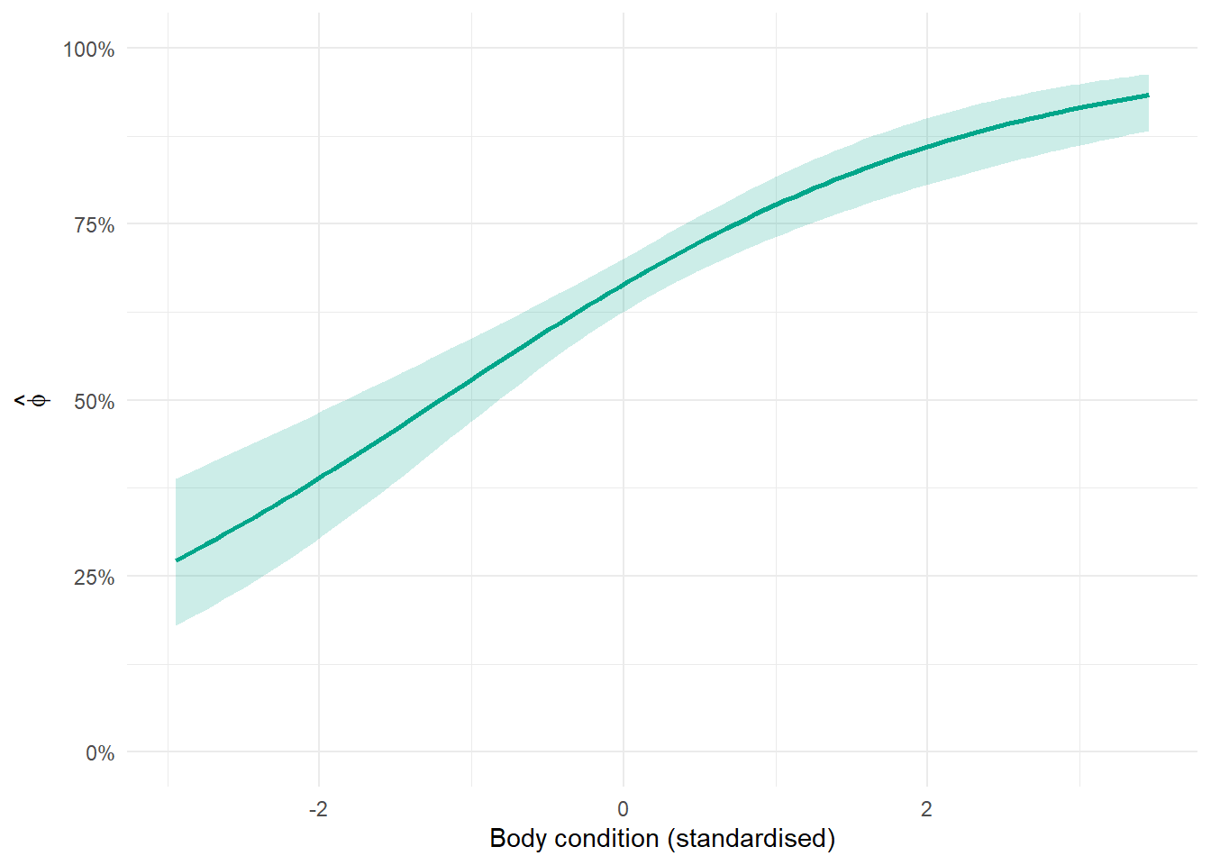
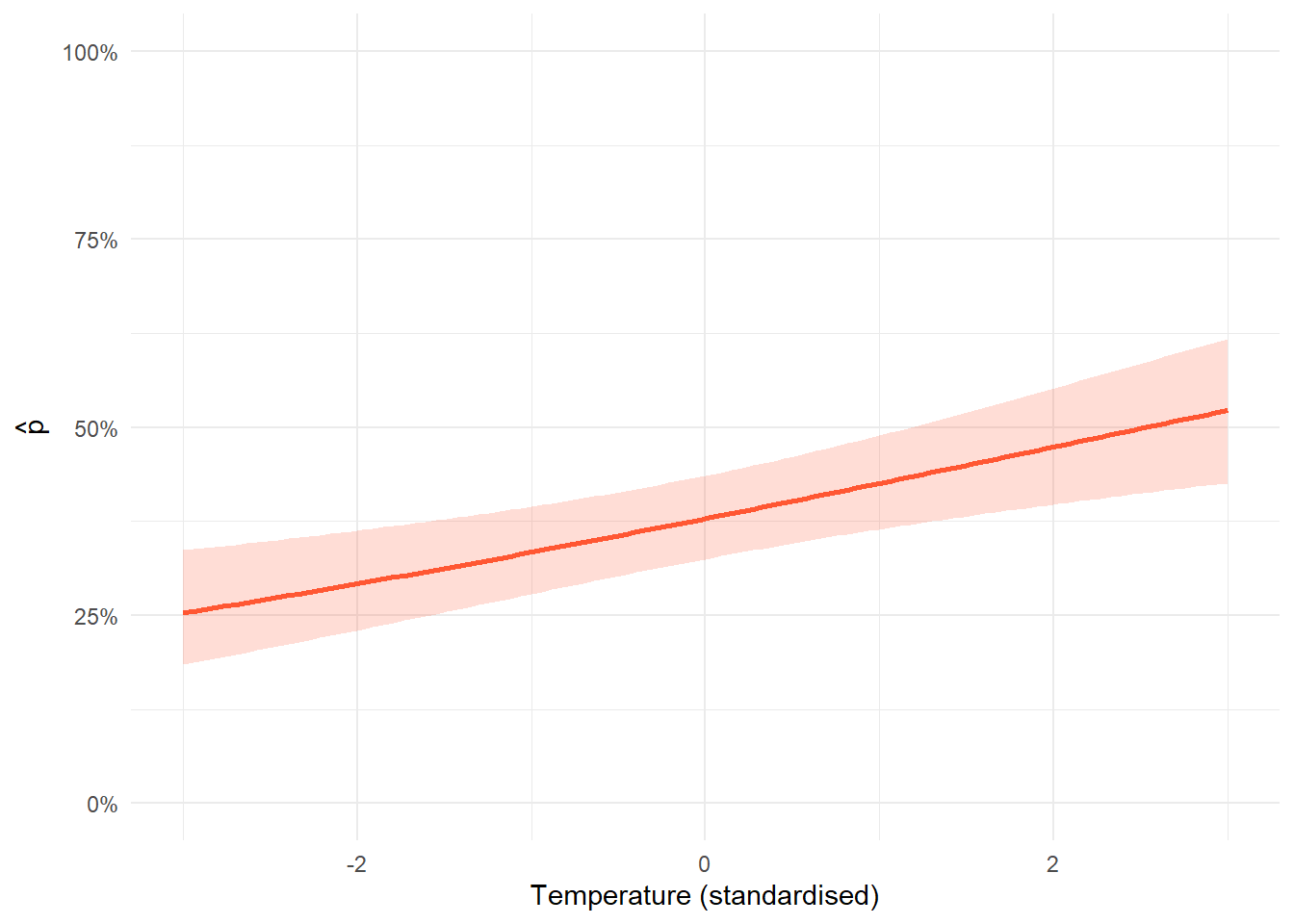
Once written like this, translating to RMark formula syntax is direct. \(\beta_0 + \beta_1 \times \text{Condition}\) becomes ~ body_cond. \(\alpha_0 + \alpha_1 \times \text{Temperature}\) becomes ~ temp. The gamma parameters are constant here, so both get ~ 1.

Fitting the model

Code

rd_processed <- process.data(
  rd_df,
  model          = "Robust",
  time.intervals = time_intervals
)

rd_ddl <- make.design.data(rd_processed)

rd_fit <- mark(
  rd_processed,
  rd_ddl,
  model.parameters = list(
    S                = list(formula = ~ body_cond),
    p                = list(formula = ~ temp),
    GammaPrime       = list(formula = ~ 1),
    GammaDoublePrime = list(formula = ~ 1)
  ),
  output = FALSE,
  silent = TRUE
)

Code

rd_fit$results$beta

                               estimate        se        lcl        ucl
S:(Intercept)                 0.6836572 0.0868179  0.5134941  0.8538204
S:body_cond                   0.5662978 0.0880560  0.3937080  0.7388876
GammaDoublePrime:(Intercept) -1.8358266 0.4107363 -2.6408698 -1.0307834
GammaPrime:(Intercept)       -1.7066375 1.6283436 -4.8981911  1.4849161
p:(Intercept)                -0.4947268 0.1207431 -0.7313832 -0.2580704
p:temp                        0.1953920 0.0539919  0.0895678  0.3012162
c:(Intercept)                -0.3779775 0.0634956 -0.5024289 -0.2535262
f0:(Intercept)                4.7518438 0.2117942  4.3367270  5.1669605
f0:session2                  -0.9039858 0.2115448 -1.3186137 -0.4893580
f0:session3                  -1.3291764 0.2481375 -1.8155260 -0.8428268
f0:session4                  -1.8007971 0.3008318 -2.3904275 -1.2111667
f0:session5                  -1.7028223 0.2828947 -2.2572959 -1.1483487
f0:session6                  -2.0558175 0.3328917 -2.7082852 -1.4033499

The beta table gives you all parameter estimates on the logit scale with standard errors and confidence intervals. The row names map directly to the model equations: S:(Intercept) is \(\beta_0\), S:body_condition is \(\beta_1\), p:(Intercept) is \(\alpha_0\), p:temp is \(\alpha_1\).

Visualising the results

The logic for every predicted relationship figure in this tutorial follows the same four steps, and once you understand them you can apply them to any parameter in any model.

Step 1: Extract the relevant coefficients from the beta table. - The beta table gives you the estimated intercept and slope for each parameter on the logit scale. For a survival model with one covariate, you need the intercept (\(\beta_0\)) and the slope (\(\beta_1\)). For detection, you need the same two things for \(\alpha_0\) and \(\alpha_1\). You also need the standard errors for both, which you will use in step 3.

Step 2: Build a sequence of covariate values and generate predictions on the logit scale. - Create a vector of evenly spaced values spanning the range of your covariate. For each value \(x\), calculate \(\beta_0 + \beta_1 \times x\). This gives you the predicted value on the logit scale across the range of the covariate.

Step 3: Calculate uncertainty using the delta method. - The confidence interval cannot be calculated by simply adding and subtracting 1.96 standard errors from the prediction, because the prediction combines two uncertain quantities: the intercept and the slope. The delta method accounts for both. The variance of \(\beta_0 + \beta_1 \times x\) on the logit scale is:

\(\text{Var} = \text{SE}_{\beta_0}^2 + x^2 \times \text{SE}_{\beta_1}^2 + 2x \times \text{Cov}(\beta_0, \beta_1)\)

The covariance term \(\text{Cov}(\beta_0, \beta_1)\) comes from the variance-covariance matrix of the model ( rd_fit$results$beta.vcv), indexed by the row and column positions of the two parameters in the beta table.

Step 4: Back-transform everything with plogis(). - The predictions and confidence interval bounds are all on the logit scale. Apply plogis() to convert them to probabilities before plotting. The lower bound is plogis(prediction - 1.96 * sqrt(variance)) and the upper bound is plogis(prediction + 1.96 * sqrt(variance)).

When you apply this to your own data, the only things that change are the covariate name, the row positions of the relevant parameters in the beta table, and the range of covariate values you predict over. The structure of the code is identical every time.

Survival as a function of body condition

Code

beta <- rd_fit$results$beta
vcv  <- rd_fit$results$beta.vcv

phi_int_est  <- beta["S:(Intercept)",    "estimate"]
phi_cond_est <- beta["S:body_cond", "estimate"]
phi_int_se   <- beta["S:(Intercept)",    "se"]
phi_cond_se  <- beta["S:body_cond", "se"]

int_idx  <- 1
cond_idx <- 2

cond_seq <- seq(min(cond_seen), max(cond_seen), length.out = 100)

# Predicted survival on logit scale
logit_phi <- phi_int_est + phi_cond_est * cond_seq

# Delta method variance on logit scale
var_logit_phi <- phi_int_se^2 +
                 cond_seq^2 * phi_cond_se^2 +
                 2 * cond_seq * vcv[int_idx, cond_idx]

phi_df <- data.frame(
  condition = cond_seq,
  phi       = plogis(logit_phi),
  lwr       = plogis(logit_phi - 1.96 * sqrt(abs(var_logit_phi))),
  upr       = plogis(logit_phi + 1.96 * sqrt(abs(var_logit_phi)))
)

ggplot(phi_df, aes(x = condition)) +
  geom_ribbon(aes(ymin = lwr, ymax = upr), fill = "#00A68A", alpha = 0.2) +
  geom_line(aes(y = phi), colour = "#00A68A", linewidth = 1) +
  scale_y_continuous(limits = c(0, 1), labels = scales::percent) +
  labs(
    x        = "Body condition (standardised)",
    y        = expression(hat(phi))
  ) +
  theme_minimal()

The confidence interval is calculated using the delta method, which propagates uncertainty from both the intercept and slope through the inverse logit transformation. The key thing to look at here is whether the interval overlaps a flat line at any particular probability: if the lower bound is clearly above or the upper bound clearly below a reference value, that is evidence of a real effect.

Detection as a function of temperature

Code

p_int_est  <- beta["p:(Intercept)", "estimate"]
p_temp_est <- beta["p:temp",        "estimate"]
p_int_se   <- beta["p:(Intercept)", "se"]
p_temp_se  <- beta["p:temp",        "se"]

p_int_idx  <- 5
p_temp_idx <- 6

temp_seq <- seq(-3, 3, length.out = 100)

logit_p <- p_int_est + p_temp_est * temp_seq

var_logit_p <- p_int_se^2 +
               temp_seq^2 * p_temp_se^2 +
               2 * temp_seq * vcv[p_int_idx, p_temp_idx]

p_df <- data.frame(
  temp = temp_seq,
  p    = plogis(logit_p),
  lwr  = plogis(logit_p - 1.96 * sqrt(abs(var_logit_p))),
  upr  = plogis(logit_p + 1.96 * sqrt(abs(var_logit_p)))
)

ggplot(p_df, aes(x = temp)) +
  geom_ribbon(aes(ymin = lwr, ymax = upr), fill = "#FF5733", alpha = 0.2) +
  geom_line(aes(y = p), colour = "#FF5733", linewidth = 1) +
  scale_y_continuous(limits = c(0, 1), labels = scales::percent) +
  labs(
    x        = "Temperature (standardised)",
    y        = expression(hat(p))
  ) +
  theme_minimal()

Population size estimates across primary periods

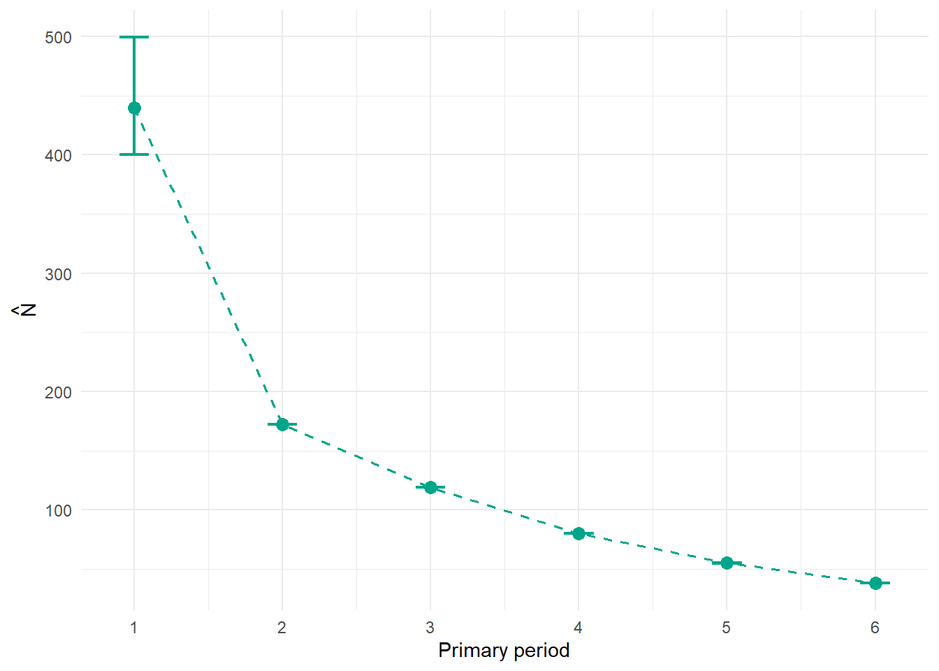
The per-period population size \(\hat{N}_t\) is one of the headline outputs of a robust design study. In RMark it is derived from the f0 parameter, which represents the estimated number of individuals that were present but never detected in each primary period. Add the observed count to f0 and you have \(\hat{N}_t\).

Code

f0_rows <- beta[grepl("^f0", rownames(beta)), ]

# Number of distinct individuals detected in each primary period
n_detected <- sapply(1:n_primary, function(t) {
  cols <- ((t - 1) * n_secondary + 1):(t * n_secondary)
  sum(rowSums(det_seen[, cols]) > 0)
})

# f0 is on log scale in RMark
f0_est <- exp(f0_rows[, "estimate"])
f0_lcl <- exp(f0_rows[, "lcl"])
f0_ucl <- exp(f0_rows[, "ucl"])

N_df <- data.frame(
  period = 1:n_primary,
  N_hat  = n_detected + f0_est,
  N_lcl  = n_detected + f0_lcl,
  N_ucl  = n_detected + f0_ucl
)

ggplot(N_df, aes(x = period, y = N_hat)) +
  geom_errorbar(aes(ymin = N_lcl, ymax = N_ucl),
                width = 0.2, colour = "#00A68A", linewidth = 0.8) +
  geom_point(size = 3, colour = "#00A68A") +
  geom_line(colour = "#00A68A", linewidth = 0.6, linetype = "dashed") +
  scale_x_continuous(breaks = 1:n_primary) +
  labs(
    x        = "Primary period",
    y        = expression(hat(N))
  ) +
  theme_minimal()

This plot shows population trend across the study corrected for imperfect detection. A declining trend here is not an artefact of getting worse at detecting animals over time: because \(p\) is estimated separately, the \(\hat{N}_t\) estimates reflect true changes in abundance. For most conservation applications this is the number you actually care about.

A note on your real data

Everything above used simulated data where we knew the true values. With your own data there are a few practical things to be careful about.

Standardise your continuous covariates. Subtract the mean and divide by the standard deviation before fitting. MARK can be numerically unstable with covariates on very different scales, and standardised coefficients are directly comparable in magnitude. This is especially important when you write up: a coefficient of 0.3 on a standardised covariate is interpretable. A coefficient of 0.003 on rainfall measured in millimetres is not.

Check for missing covariate values. RMark does not handle NA in covariates gracefully. Either impute or drop individuals with missing covariate data before calling process.data().

Make sure your time.intervals matches your data structure exactly. The most common source of cryptic errors in RMark is a mismatch between the length of the capture history strings and the length of time.intervals. Use the build_time_intervals() function above rather than constructing the vector by hand.

Keep your raw data and your RMark data frame separate. You will almost certainly need the original data again for plotting, checking, or sharing. Do not modify it in place.