How many animals are there, and are they surviving?
Two of the most fundamental questions in ecology and conservation are: how many individuals of a species are there, and how well are they surviving? How many Atlantic salmon are in the River Dee? What proportion of juveniles survive to adulthood? Is that survival rate declining? Is a conservation intervention actually working?
Lily, in your case these questions become; How many willow warblers are present at your study sites? How well are they surviving between breeding seasons? Is survival declining? Are any interventions or habitat changes making a difference?
These are not easy questions to answer, and the reason comes down to the same problem that runs through this entire tutorial: you will never see every bird that is there.
These questions sound simple but they’re not. And the reason for that comes down to a problem that seems simple but is hard to deal with.
The naive approach
Imagine I want to estimate how many otters live along a stretch of river. I go out and count them. I spot 23 otters.
So there are 23 otters?
Maybe. But I wouldn’t bet a £100 that I saw every single otter that was there. Some might’ve been in burrows. Some were maybe around the bend in the river. Some maybe saw me coming and hid. The 23 I counted is not the true population size. It is the true population size multiplied by my probability of detecting any given otter.
\[\text{Count} = N \times p\]
where \(N\) is the true number of otters and \(p\) is my detection probability. If \(p = 1\) (i.e. I have 100% chance of seeing each otter), my count equals the true population. If \(p < 1\), and it is almost always less than 1, my count is an underestimate. How badly it underestimates depends entirely on how low \(p\) is.
This is imperfect detection. This is the default condition of almost every single wildlife survey ever conducted. If you have ever counted animals in the field and assumed that count represented the true number present, you were almost certainly wrong.
Mark individuals
Here is where the “mark” part of mark-recapture comes in. The idea is pretty simple:
If you catch some animals, mark them, release them, and then go back and catch animals again, the proportion of marked animals in your second sample tells you something about how many unmarked ones you missed.
Say I catch 20 otters, tag each one with a unique ID, and release them back into the river. A week later I come back and catch another 20 otters. Of these 20, I find that 5 of them have the tags I put on a week ago. So I recaptured 5 out of the 20 I originally marked. That recapture rate of \(\frac{5}{20} = 25\%\) is an estimate of my detection probability. And if I only detected 25% of last weeks marked animals in my second sample, I probably only detected about 25% of unmarked animals too. Which means my second sample of 20 likely represents about 25% of the true population, meaning there are roughly \(\frac{20}{0.25} = 80\) otters in total.
That’s the Lincoln-Petersen estimator, and we’ll work through it properly on the next page. For now, the main idea is that recaptures allow us to figure out detection probability, which is what allows us to estimate true population size rather than just report a count and hope for the best.
All good and well but there’s actually a second problem on top of imperfect detection.
The second problem: individuals can die
Individual animals are not immortal and static. They move, disperse, and/or they die.
This matters a lot because it creates a new version of the detection problem.
Imagine I tag 50 fish in June. In August I go back and sample again. I catch 30 fish, of which 12 have tags. Fine - same as before with the otters. But now I want you to think about the 38 tagged fish I did not recapture. Those “non-recaptures” have two possible explanations:
They are still alive, I just did not catch them. My detection probability is (almost always) less than 100%, so that’s entirely plausible. (This is what we assumed above with the otters)
They are dead.
A non-recapture has two possible meanings: missed, or dead. The crap part of that: both explanations predict exactly the same observation in your data - a zero. In both cases you don’t see the fish but the biological distinction between missed and dead is obviously important…
If you cannot separate these two explanations, you cannot estimate either detection probability or survival probability reliably. They are completely tangled up in each other.
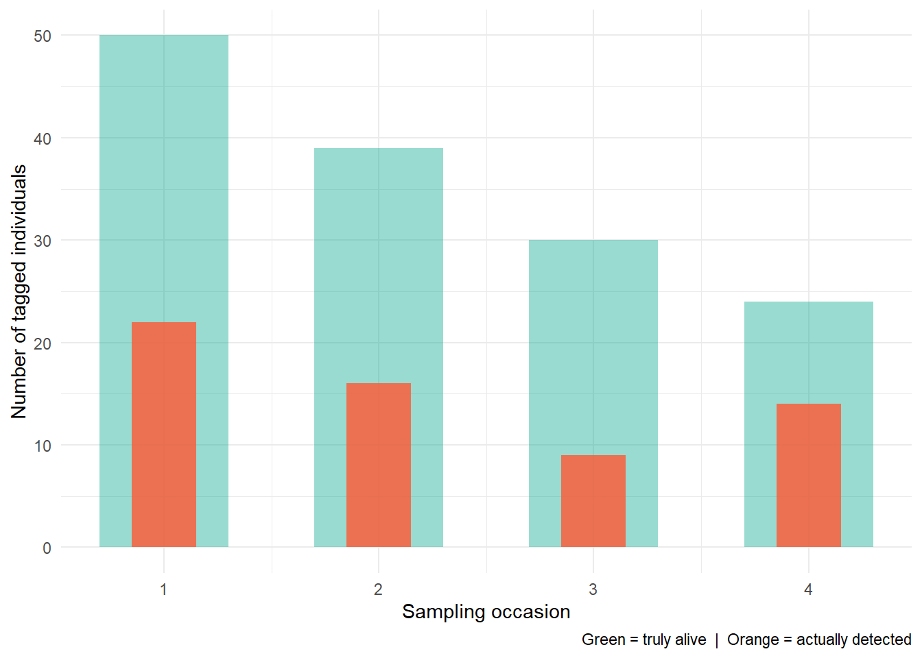
The following simulation hopefully makes this tangible (don’t worry about the code). We follow 50 tagged individuals across four sampling occasions, assuming a survival probability of 0.75 between occasions and detection probabilities that range from 0.30 to 0.80 across the four surveys.
The green bars show how many animals are truly alive at each occasion. The orange bars show how many we actually detect. The gap between them is entirely due to imperfect detection, not death. But if I only showed you the orange bars and asked you to calculate a survival rate, you’d probably conclude things look ok, but based on the green bars, this population is crashing fast.
This is where using the right stats matters a lot. Imagine this is a critically endangered population, and you’re the conservation officer. If you use basic stats you’re going to tell everyone “don’t worry, the species are doing fine. They’re stable”. In doing so, you’ve likely just condemned a species to extinction. We don’t use complicated stats for the sake of it. We use it because there’s a god damned moral imperative to make sure you make the best decision with the data you have.
Try it yourself: dead or hiding?
Before we formalise this problem, try to get a proper sense of it. Below are four tagged animals. Their detection histories are shown one occasion at a time. Each time your survey draws a blank, you must decide: was the animal dead, or was it alive and just not detected?
Code
{const animals = [ { id:"Animal #7",alive: [1,1,1,1],detected: [1,0,0,1] }, { id:"Animal #12",alive: [1,1,0,0],detected: [1,1,0,0] }, { id:"Animal #3",alive: [1,1,1,1],detected: [1,0,1,0] }, { id:"Animal #19",alive: [1,0,0,0],detected: [1,0,0,0] } ];let ai =0, occ =0, guesses = [], phase ="playing";const el =document.createElement("div"); el.style.cssText="background:#202123;border-radius:8px;padding:20px;color:#cccccc;font-family:sans-serif";functiondraw() {const a = animals[ai];const n = a.alive.length;let tiles =`<div style="display:flex;gap:8px;flex-wrap:wrap;margin-bottom:16px">`;for (let i =0; i < n; i++) {let bg="#2a2a2a", bd="#444", icon="·", sub="";if (phase ==="revealed") {if (a.detected[i]) { bg="#1a3a2a"; bd="#00A68A"; icon="✓"; sub="Detected"; }elseif (a.alive[i]) { bg="#2e2a10"; bd="#FFD700"; icon="○"; sub="Alive, missed"; }else { bg="#3a1a1a"; bd="#FF5733"; icon="✗"; sub="Dead"; } } else {if (i < occ) {if (a.detected[i]) { bg="#1a3a2a"; bd="#00A68A"; icon="✓"; sub="Detected"; }elseif (guesses[i]==="d") { bg="#3a1a1a"; bd="#FF5733"; icon="✗"; sub="You said: Dead"; }elseif (guesses[i]==="h") { bg="#2e2a10"; bd="#FFD700"; icon="?"; sub="You said: Hiding"; } } elseif (i === occ) { bg="#1a2535"; bd="#4a9eff"; icon="→"; sub="Current"; } } tiles +=`<div style="flex:1;min-width:72px;background:${bg};border:2px solid ${bd};border-radius:6px;padding:8px;text-align:center"> <div style="font-size:11px;color:#888">Occasion ${i+1}</div> <div style="font-size:22px;margin:4px 0">${icon}</div> <div style="font-size:11px;color:#aaa;min-height:14px">${sub}</div> </div>`; } tiles +=`</div>`;let action ="";if (phase ==="revealed") {const allAlive = a.alive.every(x => x ===1);const diedAt = a.alive.indexOf(0);const summary = allAlive?`<strong style="color:#00A68A">This animal was alive for all four occasions.</strong> Every non-detection was a missed observation, not a death.`:`This animal died between occasion ${diedAt} and occasion ${diedAt+1}. Non-detections before that were misses; after that, the animal was gone.`;let wrong =0, total =0;for (let i =0; i < n; i++) {if (!a.detected[i] && guesses[i] !=null) { total++;if (guesses[i] !== (a.alive[i] ?"h":"d")) wrong++; } }const verdict = total ===0?"": wrong >0?`<p style="color:#FFD700;font-size:13px;margin:8px 0 0">You got ${wrong} of ${total} guess${total>1?"es":""} wrong — and there was no way to know from the data alone. That is the point.</p>`:`<p style="color:#aaa;font-size:13px;margin:8px 0 0">You got them all right this time — but could you be certain? The data alone cannot prove it.</p>`;const nxt = ai < animals.length-1?`<button id="nxtA" style="margin-top:12px;background:#333;color:#ccc;border:1px solid #555;padding:8px 20px;border-radius:6px;cursor:pointer">Try another animal →</button>`:`<p style="color:#666;font-size:13px;margin-top:12px">You have seen all four animals. The same ambiguity lives in every zero in every dataset.</p>`; action =`<div style="background:#1a2a1a;border:1px solid #00A68A;border-radius:6px;padding:14px"> <p style="margin:0;color:#ccc;font-size:14px">${summary}</p>${verdict}</div>${nxt}`; } elseif (occ >= n) { action =`<div style="text-align:center"> <p style="color:#999;margin-bottom:10px">All occasions complete. Ready to see what actually happened?</p> <button id="revBtn" style="background:#4a9eff;color:#fff;border:none;padding:10px 24px;border-radius:6px;cursor:pointer;font-size:14px">Reveal the truth</button> </div>`; } else {if (a.detected[occ]) { action =`<div style="background:#1a3a2a;border:1px solid #00A68A;border-radius:6px;padding:14px;text-align:center"> <p style="margin:0;color:#00A68A;font-weight:bold">✓ Detected at occasion ${occ+1}!</p> <p style="margin:6px 0 0;color:#999;font-size:13px">The animal appeared in your survey. Definitely alive at this point.</p> </div> <div style="text-align:center;margin-top:12px"> <button id="nxtO" style="background:#333;color:#ccc;border:1px solid #555;padding:8px 20px;border-radius:6px;cursor:pointer">Next occasion →</button> </div>`; } else { action =`<div style="background:#252525;border:1px solid #555;border-radius:6px;padding:14px;text-align:center"> <p style="margin:0;color:#fff">Occasion ${occ+1}: <strong>not detected.</strong></p> <p style="margin:8px 0 0;color:#999;font-size:13px">Your survey drew a blank. What do you think happened to this animal?</p> </div> <div style="display:flex;gap:12px;justify-content:center;margin-top:12px"> <button id="dBtn" style="background:#3a1a1a;color:#FF5733;border:2px solid #FF5733;padding:10px 28px;border-radius:6px;cursor:pointer;font-weight:bold">✗ Dead</button> <button id="hBtn" style="background:#2e2a10;color:#FFD700;border:2px solid #FFD700;padding:10px 28px;border-radius:6px;cursor:pointer;font-weight:bold">? Hiding</button> </div>`; } } el.innerHTML=` <div style="display:flex;justify-content:space-between;align-items:center;margin-bottom:10px"> <h3 style="margin:0;color:#fff">${a.id} — Dead or hiding?</h3> <span style="font-size:12px;color:#666">${ai+1} / ${animals.length}</span> </div> <p style="color:#999;font-size:13px;margin-bottom:14px">Tagged and released at occasion 1. Watch each survey unfold. When there is a non-detection, make your call.</p>${tiles}${action}`; el.querySelector("#nxtO")?.addEventListener("click", () => { guesses[occ]=null; occ++;draw(); }); el.querySelector("#dBtn")?.addEventListener("click", () => { guesses[occ]="d"; occ++;draw(); }); el.querySelector("#hBtn")?.addEventListener("click", () => { guesses[occ]="h"; occ++;draw(); }); el.querySelector("#revBtn")?.addEventListener("click",() => { phase="revealed";draw(); }); el.querySelector("#nxtA")?.addEventListener("click", () => { ai++; occ=0; guesses=[]; phase="playing";draw(); }); }draw();return el;}
The problem
To describe these two competing explanations precisely, we need to name two quantities. The first is \(p\), the probability of detecting an individual that is alive and present during a survey. The second is \(\phi\) (the Greek letter “phi”), the probability an individual survives from one survey to the next. These two quantities sit at the heart of everything that follows in this tutorial.
When you do not recapture a tagged animal, you are facing two competing hypotheses:
Hypothesis A: The animal is alive but you missed it. This happens with probability \(\phi \times (1 - p)\): the animal survived (\(\phi\)) the interval between surveys but you failed to detect it (\(1 - p\), the probability of not seeing it).
Hypothesis B: The animal is dead. This happens with probability \(1 - \phi\): the animal did not survive the time between surveys.
Both predict the same observation; 0. When all you have is a capture occasion you cannot tell them apart. Use the sliders below to explore how the balance between these two explanations shifts depending on the true values of \(\phi\) and \(p\).
Code
viewof phi_bar = Inputs.range([0.05,0.99], {value:0.75,step:0.01,label:"Survival probability (\u03c6)"})
Code
viewof p_bar = Inputs.range([0.05,0.99], {value:0.40,step:0.01,label:"Detection probability (p)"})
Code
{const data = [ { scenario:"Alive, not detected",prob: phi_bar * (1- p_bar) }, { scenario:"Dead",prob:1- phi_bar } ];const winner = data[0].prob> data[1].prob?"alive but missed":"dead";const winColor = winner ==="alive but missed"?"#00A68A":"#FF5733";const chart = Plot.plot({style: { background:"#202123",color:"#cccccc",fontSize:"13px" },marginLeft:160,width:520,height:160,x: { label:"Probability",tickFormat:"%",domain: [0,1],grid:true },y: { label:null },color: {domain: ["Alive, not detected","Dead"],range: ["#00A68A","#FF5733"] },marks: [ Plot.barX(data, { y:"scenario",x:"prob",fill:"scenario" }), Plot.ruleX([0], { stroke:"#444" }) ] });returnhtml`<div style="background:#202123;padding:12px;border-radius:6px">${chart} <p style="font-size:13px;color:#999;margin:10px 0 0"> With these values, a non-detection is more likely explained by <strong style="color:${winColor}">${winner}</strong>. Try adjusting both sliders \u2014 notice how easily this conclusion flips, and how different combinations of \u03c6 and p can make a healthy population look like a collapsing one, or vice versa. </p> </div>`;}
This is why a single survey with recaptures is not enough. You need a framework that estimates \(\phi\) and \(p\) simultaneously, using the full pattern of detections and non-detections across multiple occasions to untangle them.
What we need to make progress
To estimate survival and detection simultaneously, rather than having them hopelessly tangled together, we need three things.
First, individually marked animals. Not just a count of how many we saw, but a record of which specific individuals we saw on each occasion. This is what allows us to track fates through time rather than just tallying up numbers.
Second, multiple sampling occasions. A single occasion gives us a count. Multiple occasions give us a pattern of detections and non-detections across time, and that pattern contains the information we need to estimate both \(\phi\) and \(p\) separately.
Third, a model that represents both processes explicitly. One that says, formally, that observing an animal requires both that it survived to the next occasion and that we actually detected it, and uses that structure to estimate each parameter on its own terms. If you have worked through the GLM refresher, you already have the statistical foundation for this. The models we will build are extensions of that same framework — they simply need to account for these two processes, survival and detection, at the same time.
The next page introduces the simplest version of this thinking: the Lincoln-Petersen estimator. It does not quite tick all three boxes but it builds the intuition clearly and cleanly before we move on to models that do.