The Robust Design

The problem we are stuck with

Let us take stock of where we are.

The Lincoln-Petersen estimator gives us population size \(N\), but only under closure. The population cannot change between your two sampling occasions. That assumption is fine over a day or two. Over weeks or months it becomes fiction.

The Cormack-Jolly-Seber model gives us apparent survival \(\phi\), but it requires the population to be open. Animals can die between occasions, which is precisely what we are trying to estimate. In exchange for that realism, CJS conditions on marked individuals only and cannot estimate \(N\) at all.

So we have two models. One estimates \(N\) but cannot handle survival. The other estimates survival but cannot estimate \(N\). What we actually want is both, from the same study, at the same time.

This is not a minor inconvenience. For most real conservation questions you need both. How many individuals are there and are they surviving well enough to maintain that number? Neither question makes much sense without the other.

The robust design, introduced by Kenneth Pollock in 1982, resolves this tension with an idea that is almost frustratingly simple once you see it.

The key insight: two time scales

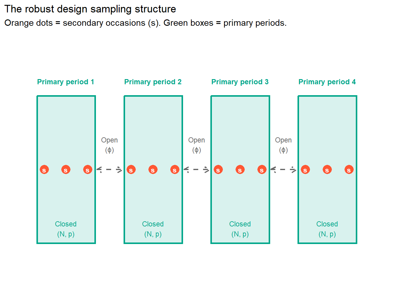
The reason LP and CJS are in conflict is that they need opposite things from the population. LP needs closure. CJS needs openness. The robust design gives each of them what they need by operating at two different time scales simultaneously.

Here is the structure:

Code

library(ggplot2)
library(dplyr)

# Primary periods
primary <- data.frame(
  x_start = c(1, 4, 7, 10),
  x_end   = c(3, 6, 9, 12),
  y = 0.5,
  label = paste("Primary period", 1:4)
)

# Secondary occasions within each primary period
secondary <- data.frame(
  x = c(1.25, 2, 2.75,
         4.25, 5, 5.75,
         7.25, 8, 8.75,
         10.25, 11, 11.75),
  y = 0.5,
  primary = rep(1:4, each = 3)
)

# Open arrows between primary periods
arrows_df <- data.frame(
  x    = c(3.05, 6.05, 9.05),
  xend = c(3.95, 6.95, 9.95),
  y = 0.5
)

ggplot() +
  # Primary period boxes
  geom_rect(data = primary,
            aes(xmin = x_start, xmax = x_end,
                ymin = 0.15, ymax = 0.85),
            fill = "#00A68A", alpha = 0.15, colour = "#00A68A", linewidth = 1) +
  # Primary period labels
  geom_text(data = primary,
            aes(x = (x_start + x_end) / 2, y = 0.92, label = label),
            size = 3.2, colour = "#00A68A", fontface = "bold") +
  # Secondary occasion points
  geom_point(data = secondary,
             aes(x = x, y = y),
             size = 5, colour = "#FF5733") +
  geom_text(data = secondary,
            aes(x = x, y = y),
            label = "s", size = 3, colour = "white", fontface = "bold") +
  # Open arrows between primary periods
  geom_segment(data = arrows_df,
               aes(x = x, xend = xend, y = y, yend = y),
               arrow = arrow(length = unit(0.25, "cm"), ends = "both"),
               linewidth = 0.8, colour = "grey40", linetype = "dashed") +
  # Labels for arrows
  annotate("text", x = c(3.5, 6.5, 9.5), y = 0.62,
           label = "Open\n(\u03d5)", size = 3, colour = "grey40") +
  # Closed label inside boxes
  annotate("text", x = c(2, 5, 8, 11), y = 0.22,
           label = "Closed\n(N, p)", size = 3, colour = "#00A68A") +
  scale_x_continuous(limits = c(0.5, 13)) +
  scale_y_continuous(limits = c(0, 1.1)) +
  labs(x = NULL, y = NULL,
       title = "The robust design sampling structure",
       subtitle = "Orange dots = secondary occasions (s). Green boxes = primary periods.") +
  theme_minimal() +
  theme(axis.text = element_blank(),
        panel.grid = element_blank())

The primary periods are separated by long enough gaps that the population can change between them. Animals can die. Animals can be recruited. This is the open part, handled by CJS-style logic, and it gives us \(\phi\).

The secondary occasions are the repeated sampling events within each primary period, conducted close enough together in time that we can reasonably assume the population is closed during that window. No births, no deaths, no permanent movement in or out. This is the closed part, handled by LP-style logic, and it gives us \(N\).

The robust design nests one inside the other. Closure within primary periods. Openness between them. LP and CJS stop being in conflict because they are now operating at different time scales.

That is the entire conceptual insight. Everything else is working out the details.

The data structure

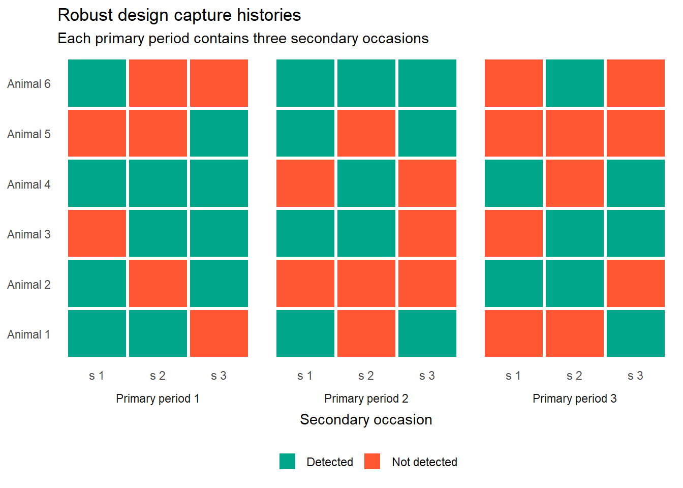
The data structure follows directly from the sampling structure. Each individual now has a capture history that operates at two levels.

At the between-period level, there is a summary detection for each primary period: was the animal detected at least once during that primary period, yes or no? This is the coarse-grained history that feeds the open-population (survival) component of the model.

At the within-period level, there is a detailed detection history across the secondary occasions within each primary period. This fine-grained history feeds the closed-population (abundance and detection) component.

Code

set.seed(7)

# 6 animals, 3 primary periods, 3 secondary occasions each
animals <- paste0("Animal ", 1:6)
periods <- paste0("P", rep(1:3, each = 3), "_s", rep(1:3, times = 3))

ch_matrix <- matrix(
  c(1,1,0, 1,0,1, 0,0,1,
    1,0,1, 0,0,0, 1,1,0,
    0,1,1, 1,1,0, 0,1,1,
    1,1,1, 0,1,0, 1,0,1,
    0,0,1, 1,0,1, 0,0,0,
    1,0,0, 1,1,1, 0,1,0),
  nrow = 6, byrow = TRUE
)

colnames(ch_matrix) <- periods
rownames(ch_matrix) <- animals

ch_df <- as.data.frame(ch_matrix) |>
  tibble::rownames_to_column("animal") |>
  tidyr::pivot_longer(-animal, names_to = "occasion", values_to = "detected") |>
  mutate(
    primary = as.integer(substr(occasion, 2, 2)),
    secondary = as.integer(substr(occasion, 5, 5)),
    detected_label = if_else(detected == 1, "Detected", "Not detected")
  )

ggplot(ch_df, aes(x = secondary, y = animal, fill = detected_label)) +
  geom_tile(colour = "white", linewidth = 1.2) +
  facet_grid(~ paste("Primary period", primary),
             switch = "x") +
  scale_fill_manual(values = c("Detected" = "#00A68A",
                                "Not detected" = "#FF5733")) +
  scale_x_continuous(breaks = 1:3, labels = paste("s", 1:3)) +
  labs(x = "Secondary occasion", y = NULL, fill = NULL,
       title = "Robust design capture histories",
       subtitle = "Each primary period contains three secondary occasions") +
  theme_minimal() +
  theme(legend.position = "bottom",
        panel.grid = element_blank(),
        strip.placement = "outside")

Every red tile carries the same ambiguity as before. But now there are two levels at which that ambiguity operates, and the model deals with each one separately.

Within a primary period, a red tile means the animal was alive and present but not detected. The population is assumed closed so death and emigration are ruled out. The only explanation is imperfect detection.

Between primary periods, a zero summary (never detected across any secondary occasion in a primary period) could mean the animal died before that period, or that it was alive but never detected across any of the secondary occasions. The open-population component of the model handles that ambiguity, just as CJS did.

Building the likelihood

The robust design likelihood separates cleanly into two parts that are estimated together but can be understood separately. We will build each one up in turn.

Part 1: Within primary periods (closed population)

Within each primary period, the population is closed. We have repeated secondary occasions and we want to estimate two things: detection probability \(p\) and population size \(N_t\) for that period.

This is essentially a closed-population mark-recapture model. The simplest version, sometimes called \(M_0\), assumes every individual has the same detection probability \(p\) on every secondary occasion. The probability of an individual’s within-period detection history \(\mathbf{x}_{it} = (x_{it1}, x_{it2}, \ldots, x_{its})\) across \(s\) secondary occasions, given the animal is present, is:

\[\Pr(\mathbf{x}_{it} \mid \text{present}) = \prod_{j=1}^{s} p^{x_{itj}} (1-p)^{1-x_{itj}}\]

This is just a Bernoulli product. For each secondary occasion, the animal was either detected (\(x = 1\), probability \(p\)) or not (\(x = 0\), probability \(1-p\)).

The probability of not being detected at all during a primary period, across all \(s\) secondary occasions, is:

\[1 - \tilde{p}_t = (1-p)^s\]

So the probability of being detected at least once during primary period \(t\) is:

\[\tilde{p}_t = 1 - (1-p)^s\]

This \(\tilde{p}_t\) is the effective detection probability for the whole primary period. It is the probability that links the within-period model to the between-period model. Notice that even if \(p\) is modest on any single occasion, \(\tilde{p}_t\) can be quite high if you have enough secondary occasions. This is one of the practical benefits of repeated sampling within a period.

To estimate \(N_t\), we use a Huggins-style conditional likelihood (which you don’t need to remember). The important thing is that rather than estimating \(N_t\) directly in the likelihood, we condition on the animals that were detected at least once, estimate \(p\) from their detection histories, and then derive (meaning “figure out”) \(\hat{N}_t\) afterwards as:

\[\hat{N}_t = \frac{n_t}{\hat{\tilde{p}}_t}\]

where \(n_t\) is the number of distinct individuals caught in primary period \(t\). This is Lincoln-Petersen logic in a more general form: we observed \(n_t\) animals, and we estimated that each had a \(\hat{\tilde{p}}_t\) chance of being detected, so the implied population size is \(n_t\) divided by that probability.

Part 2: Between primary periods (open population)

Between primary periods, the CJS machinery takes over. For each individual, we have a between-period capture history summarised as whether they were detected at all in each primary period (\(\omega_{it} = 1\) if detected in any secondary occasion in period \(t\), 0 otherwise).

The between-period likelihood is exactly the CJS likelihood from the previous page, but with one modification: the detection probability entering the CJS component is not the raw \(p\) from a single occasion but the effective detection probability \(\tilde{p}_t\) from the closed-population component.

\[\Pr(\omega_{it} = 1 \mid \text{alive at } t) = \tilde{p}_t\]

\[\Pr(\omega_{it} = 0 \mid \text{alive at } t) = 1 - \tilde{p}_t\]

The survival probability \(\phi_t\) operates between primary periods, exactly as in CJS:

\[z_{i,t} \sim Bernoulli(\phi_{t-1} \times z_{i,t-1})\]

And the probability of the between-period summary detection, given the true state, is:

\[\omega_{i,t} \sim Bernoulli(\tilde{p}_t \times z_{i,t})\]

The probability of never being seen again from primary period \(t\) onwards, \(\chi_t\), follows the same recursion as before but now uses \(\tilde{p}_t\) in place of the single-occasion \(p\):

\[\chi_T = 1\]

\[\chi_t = (1 - \phi_t) + \phi_t (1 - \tilde{p}_{t+1}) \chi_{t+1}\]

The full likelihood

The full robust design likelihood is the product of the two parts:

\[\mathcal{L} = \mathcal{L}_{\text{open}}(\phi, \tilde{p}) \times \prod_{t=1}^{T} \mathcal{L}_{\text{closed},t}(p_t)\]

The closed-population component is estimated separately within each primary period and delivers \(\hat{p}_t\) and \(\hat{N}_t\). The open-population component uses \(\tilde{p}_t\) derived from \(\hat{p}_t\) and delivers \(\hat{\phi}_t\). The two parts talk to each other through \(\tilde{p}_t\), which is the bridge between the two time scales.

What we can now estimate

The robust design delivers parameters that neither LP nor CJS could provide alone:

Parameter	Symbol	Source
Population size at each primary period	\(N_t\)	Closed component
Detection probability (single occasion)	\(p\)	Closed component
Effective detection probability (per primary period)	\(\tilde{p}_t\)	Derived from \(p\) and \(s\)
Apparent survival between primary periods	\(\phi_t\)	Open component
Population growth rate	\(\lambda_t = N_{t+1}/N_t\)	Derived from \(N_t\)

\(\lambda_t\) is perhaps the most practically useful derived quantity of all. It tells you directly whether the population is growing, stable, or declining between primary periods, and it is estimated honestly, accounting for imperfect detection at both the secondary occasion level and the primary period level.

A small simulation

Let us simulate a robust design dataset and get a feel for how the parameter estimates behave. We will use six primary periods with three secondary occasions each, and keep everything simple with constant \(\phi\) and \(p\). Six primary periods gives the model five survival intervals to work with, which is enough to estimate \(\phi\) reliably.

Be aware that I’m going to use a package called RMark for the modelling here. I’ll come back to this later on, but just know that it requires another piece of software, called program MARK, to be installed in order to run. You can find it here if you want to download and install it now.

Code

library(RMark)

set.seed(1988)

N_true      <- 300    # Initial population size
phi_true    <- 0.80   # Survival between primary periods
p_true      <- 0.40   # Detection on each secondary occasion
n_primary   <- 6
n_secondary <- 3

# Effective detection probability per primary period
p_tilde <- 1 - (1 - p_true)^n_secondary

cat("True N:", N_true,
    "\nTrue phi:", phi_true,
    "\nTrue p (single occasion):", p_true,
    "\nEffective p per primary period:", round(p_tilde, 3))

True N: 300 
True phi: 0.8 
True p (single occasion): 0.4 
Effective p per primary period: 0.784

Code

# Simulate capture histories
sim_robust <- function(N, phi, p, n_prim, n_sec, seed = 1988) {
  set.seed(seed)
  
  # True alive state across primary periods
  alive <- matrix(0, nrow = N, ncol = n_prim)
  alive[, 1] <- 1
  for (t in 2:n_prim) {
    alive[, t] <- rbinom(N, 1, alive[, t - 1] * phi)
  }
  
  # Detection history: N x (n_prim * n_sec)
  det <- matrix(0, nrow = N, ncol = n_prim * n_sec)
  for (t in 1:n_prim) {
    for (s in 1:n_sec) {
      col <- (t - 1) * n_sec + s
      det[, col] <- rbinom(N, 1, alive[, t] * p)
    }
  }
  
  # Keep only animals detected at least once
  det[rowSums(det) > 0, ]
}

ch_data <- sim_robust(N_true, phi_true, p_true, n_primary, n_secondary)

ch_strings <- apply(ch_data, 1, paste, collapse = "")
rd_df <- data.frame(ch = ch_strings, stringsAsFactors = FALSE)

cat("Number of individuals detected at least once:", nrow(rd_df), "\n")

Number of individuals detected at least once: 281 

Code

cat("First 10 capture histories:\n")

First 10 capture histories:

Code

head(ch_strings, 10)

 [1] "101101100010111110" "000001101111100001" "111111000000011000"
 [4] "001100000000000000" "110101011110011101" "100010000000000000"
 [7] "010011110000000000" "000101010001000110" "100000000000000000"
[10] "110100100100000000"

Code

# Process data for robust design in RMark
# time.intervals: 0 = within primary period (closed), 1 = between primary periods (open)
# 6 primary periods x 3 secondary occasions = 18 columns
# Intervals: 0 0 | 1 | 0 0 | 1 | 0 0 | 1 | 0 0 | 1 | 0 0 | 1 | 0 0
time_intervals <- c(0, 0, 1, 0, 0, 1, 0, 0, 1, 0, 0, 1, 0, 0, 1, 0, 0)

rd_processed <- process.data(rd_df,
                              model = "Robust",
                              time.intervals = time_intervals)

rd_ddl <- make.design.data(rd_processed)

# Fit model with constant phi and p, no temporary emigration
# GammaPrime and GammaDoublePrime fixed to -10 on logit scale (effectively zero)
# We will deal with temporary emigration properly on the next page
rd_fit <- mark(rd_processed, rd_ddl,
               model.parameters = list(
                 S              = list(formula = ~ 1),
                 p              = list(formula = ~ 1),
                 GammaPrime     = list(formula = ~ 1, fixed = -10),
                 GammaDoublePrime = list(formula = ~ 1, fixed = -10)
               ),
               output = FALSE,
               silent = TRUE)

Code

beta <- rd_fit$results$beta

phi_est <- plogis(beta["S:(Intercept)", "estimate"])
phi_lcl <- plogis(beta["S:(Intercept)", "estimate"] -
                    1.96 * beta["S:(Intercept)", "se"])
phi_ucl <- plogis(beta["S:(Intercept)", "estimate"] +
                    1.96 * beta["S:(Intercept)", "se"])

p_est <- plogis(beta["p:(Intercept)", "estimate"])
p_lcl <- plogis(beta["p:(Intercept)", "estimate"] -
                  1.96 * beta["p:(Intercept)", "se"])
p_ucl <- plogis(beta["p:(Intercept)", "estimate"] +
                  1.96 * beta["p:(Intercept)", "se"])

cat("Survival estimate (true =", phi_true, "):",
    round(phi_est, 3),
    "  95% CI:", round(phi_lcl, 3), "to", round(phi_ucl, 3))

Survival estimate (true = 0.8 ): 0.781   95% CI: 0.75 to 0.809

Code

cat("\nDetection estimate (true =", p_true, "):",
    round(p_est, 3),
    "  95% CI:", round(p_lcl, 3), "to", round(p_ucl, 3))

Detection estimate (true = 0.4 ): 0.025   95% CI: 0.024 to 0.026

The estimates should land reasonably close to the true values. They will not be exact because we are working with a simulated sample, but the true values should sit comfortably within the confidence intervals.

What is still missing

The model above fixes temporary emigration to zero, which is a simplification we have made deliberately. In reality, animals may temporarily leave your study area between primary periods and return later. They are not dead and not permanently gone, but during their absence they cannot be detected, which creates yet another flavour of ambiguous non-detection.

This is temporary emigration, captured by the parameters \(\gamma'\) and \(\gamma''\) (gamma prime and gamma double prime) that we have quietly set aside here. It is the subject of the next page.

For now, the important thing is that you have the core structure. Closure within primary periods gives you \(N_t\) and \(p\). Openness between primary periods gives you \(\phi\). The two time scales work together through \(\tilde{p}_t\). That structure is the robust design.