Refresher: GLMs and What They Actually Estimate

A year is a long time

Cast your mind back to when I taught you GLMs. I know, I know. It feels like another lifetime. You were younger, more innocent, and blissfully unaware that statistics would follow you into your honours year. Well, here we are.

The good news is that everything we are going to do in this tutorial series is built on top of what you already know. The robust design mark-recapture model, which sounds terrifying, is in its bones just a collection of GLMs talking to each other. So before we get anywhere near that, it is worth making sure the foundations are solid.

This page is not going to teach you anything new. It is going to remind you of something old, but with a bit more attention paid to what a GLM is actually doing, which I suspect got lost somewhere between the lecture and the exam.

What is a GLM doing?

At its core, a GLM is estimating a parameter from data.

That word, parameter, is doing a lot of work here and it is worth sitting with it for a moment. A parameter is a number that describes something true about the world. The average height of adult humans is a parameter. The probability that a flipped coin lands heads is a parameter. These are fixed, real values that exist whether or not we ever collect data on them.

The problem is that we can never actually know these values. We can only estimate them from data. That is the entire job of statistics, and it is the entire job of a GLM.

So when you run a GLM, you are not calculating a fact. You are making an educated guess about a parameter, with some measure of how confident you are in that guess. Keep that in mind, because it becomes crucial later.

A concrete example

Let’s say I want to know the probability that a particular species of fish is present in a lake. I survey 20 lakes and record whether the fish is there or not.

Code

set.seed(42)

n_lakes <- 20
lakes <- data.frame(
  lake = 1:n_lakes,
  fish = rbinom(n = n_lakes, size = 1, prob = 0.65)
)

lakes

   lake fish
1     1    0
2     2    0
3     3    1
4     4    0
5     5    1
6     6    1
7     7    0
8     8    1
9     9    0
10   10    0
11   11    1
12   12    0
13   13    0
14   14    1
15   15    1
16   16    0
17   17    0
18   18    1
19   19    1
20   20    1

Each row is a lake. fish is 1 if I detected the fish, and 0 if I didn’t. Pretty simple.

Now, I want to know: what is the probability that any given lake contains fish?

I could just take the mean of the fish column:

Code

mean(lakes$fish)

[1] 0.5

And honestly, for this simple case, that would give me a reasonable estimate. But the moment I want to ask why some lakes have fish and others don’t, or the moment I want to include any uncertainty in a principled way, I need a model.

Here is the model:

\[ y_i \sim Bernoulli(p_i) \\ \]

\[ logit(p_i) = \beta_0 \]

where:

• \(y\) is our observation (fish present or absent in lake \(i\))

• \(i\) is an index for which lake we are talking about

• \(\sim\) means “is generated according to”

• \(Bernoulli\) is a distribution that produces only 0 or 1

• \(p\) is the probability of detecting fish. This is our parameter. It is what we are trying to estimate.

• \(logit\) is a link function. It is a small piece of maths that keeps \(p\) between 0 and 1, because probabilities cannot be negative or greater than 1. Specifically, \(logit(p) = log\left(\frac{p}{1-p}\right)\)

• \(\beta_0\) is the intercept. Because there are no other covariates in this model, \(\beta_0\) encodes the average probability of detecting fish (on the logit scale).

Let’s fit it:

Code

mod <- glm(fish ~ 1,
           data = lakes,
           family = binomial)

summary(mod)

Call:
glm(formula = fish ~ 1, family = binomial, data = lakes)

Coefficients:
            Estimate Std. Error z value Pr(>|z|)
(Intercept)   0.0000     0.4472       0        1

(Dispersion parameter for binomial family taken to be 1)

    Null deviance: 27.726  on 19  degrees of freedom
Residual deviance: 27.726  on 19  degrees of freedom
AIC: 29.726

Number of Fisher Scoring iterations: 2

The estimate for (Intercept) (i.e. \(\beta_0\)) is on the logit scale. To convert it back to a probability that a human can understand, we use plogis():

Code

plogis(coef(mod))

(Intercept) 
        0.5 

So the model estimates roughly a 65% chance of fish being present in any given lake. Given we simulated the data with a true probability of 65%, that is reassuringly close.

Why bother with a GLM at all?

Fair question. If we can just take mean(lakes$fish), why bother?

Two reasons.

First, mean() breaks the moment you want to include covariates. If you want to ask “how does lake depth affect fish presence?”, you cannot do that with a mean. You need a model.

Second, and more importantly for our purposes: a GLM gives you uncertainty. Not just a point estimate, like 65%, but a sense of how confident you should be in that estimate. Look at the Std. Error in the summary output, and look at the 95% confidence intervals:

Code

plogis(confint(mod))

    2.5 %    97.5 % 
0.2909703 0.7090297 

The model is not just saying “65%”. It is saying “somewhere between roughly 29% and 71%, and our best guess is 65%”. That range is information. Ignoring it is how you end up overconfident.

This idea of carrying uncertainty forward is going to matter a great deal when we get to the robust design. For now, just note that a GLM gives you both an estimate and a measure of how much to trust it.

Adding a covariate

Let’s make things slightly more realistic. Maybe fish are more likely to be present in deeper lakes. I will simulate some depth data and refit the model.

Code

set.seed(42)

lakes$depth <- rnorm(n_lakes, mean = 5, sd = 2)

true_beta0 <- -1
true_beta1 <- 0.5

log_odds <- true_beta0 + true_beta1 * lakes$depth
lakes$fish <- rbinom(n_lakes, size = 1, prob = plogis(log_odds))

mod2 <- glm(fish ~ depth,
            data = lakes,
            family = binomial)

summary(mod2)

Call:
glm(formula = fish ~ depth, family = binomial, data = lakes)

Coefficients:
            Estimate Std. Error z value Pr(>|z|)  
(Intercept)  -1.5973     1.4502  -1.101   0.2707  
depth         0.5679     0.2940   1.931   0.0534 .
---
Signif. codes:  0 '***' 0.001 '**' 0.01 '*' 0.05 '.' 0.1 ' ' 1

(Dispersion parameter for binomial family taken to be 1)

    Null deviance: 22.493  on 19  degrees of freedom
Residual deviance: 16.708  on 18  degrees of freedom
AIC: 20.708

Number of Fisher Scoring iterations: 5

Now we have two parameters: \(\beta_0\) (the intercept) and \(\beta_1\) (the effect of depth). Our model is now:

\[ y_i \sim Bernoulli(p_i) \\ \]

\[ logit(p_i) = \beta_0 + \beta_1 \times Depth_i \]

The interpretation of \(\beta_1\) on the logit scale is not particularly intuitive, but we can visualise the predicted relationship to make it concrete:

Code

library(ggplot2)

depth_seq <- seq(from = min(lakes$depth),
                 to = max(lakes$depth),
                 length.out = 100)

pred_df <- data.frame(
  depth = depth_seq,
  pred = plogis(coef(mod2)[1] + coef(mod2)[2] * depth_seq)
)

ggplot() +
  geom_jitter(data = lakes,
              aes(x = depth, y = fish),
              width = 0, height = 0.02,
              alpha = 0.5) +
  geom_line(data = pred_df,
            aes(x = depth, y = pred),
            colour = "#00A68A", linewidth = 1) +
  scale_y_continuous(labels = scales::percent,
                     limits = c(0, 1)) +
  labs(x = "Lake depth (m)",
       y = "Predicted probability\nof fish presence") +
  theme_minimal()

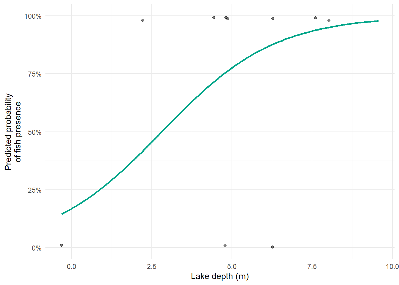
The green line is our model’s prediction. Deeper lakes are estimated to have a higher probability of containing fish, which is what we put into the simulation. The model has recovered the pattern from the data.

The thing I really want you to take away from this page

Here it is:

A GLM estimates a parameter from data. A parameter is a probability, a rate, a mean, or some other property of the world that we cannot observe directly. The GLM gives us our best guess at that parameter, plus some honest accounting of how uncertain that guess is.

That is it. That is the whole page, really.

Everything in mark-recapture, and specifically everything in the robust design, follows this exact logic. We will have parameters for survival probability. Parameters for detection probability. Parameters for population size. None of these are things we observe directly in the field. All of them are things we estimate from data, using models that are, at their core, just GLMs.

The complexity of what is coming is not in the mathematics. It is in the biology that each parameter is trying to represent, and in making sure we have set the model up in a way that lets us estimate each one without getting them confused with each other.

That last part, not getting parameters confused with each other, is actually the central challenge of mark-recapture. We will get into why on the next page.

Quick recap

Before moving on, the things worth having firmly in your head:

• A GLM estimates parameters (probabilities, means, rates) from data

• It uses a link function (like logit) to keep predictions on a sensible scale

• It gives you a point estimate and uncertainty

• Adding covariates lets you ask why a parameter varies across observations

• The plogis() function converts logit-scale estimates back to probabilities

If any of that felt shaky, now is a good time to re-read it. The rest of the tutorial series assumes this is solid.